Linear Regression

LINEAR REGRESSION

Introduction:

Linear regression attempts to model the relationship between the independent variables and a dependent variable by fitting a linear equation to the observed data.

From a machine learning context, it is the simplest model one can try out on your data. If you have a hunch that the data follows a straight-line trend, linear regression can give you quick and reasonably accurate results.  

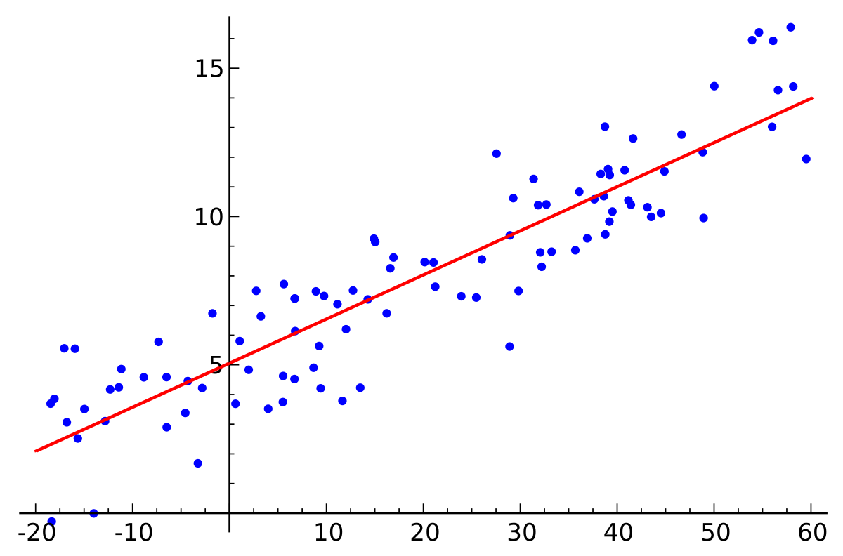
Let's consider regression with 1 independent variable and 1 dependent variable, as shown in the plot below. The blue points below represent the data we have, while the red line is the line of best fit or the regression line. 

Notation:

Keep in mind that for regression, we need to have labelled data, i.e. we need all the independent variables' and the dependent variable's values to be given. Consider a simple regression case in which we are trying to predict the price of a house from multiple features such as size, number of rooms, number of floors, etc.  

Please go through the notation given in the picture below thoroughly. 

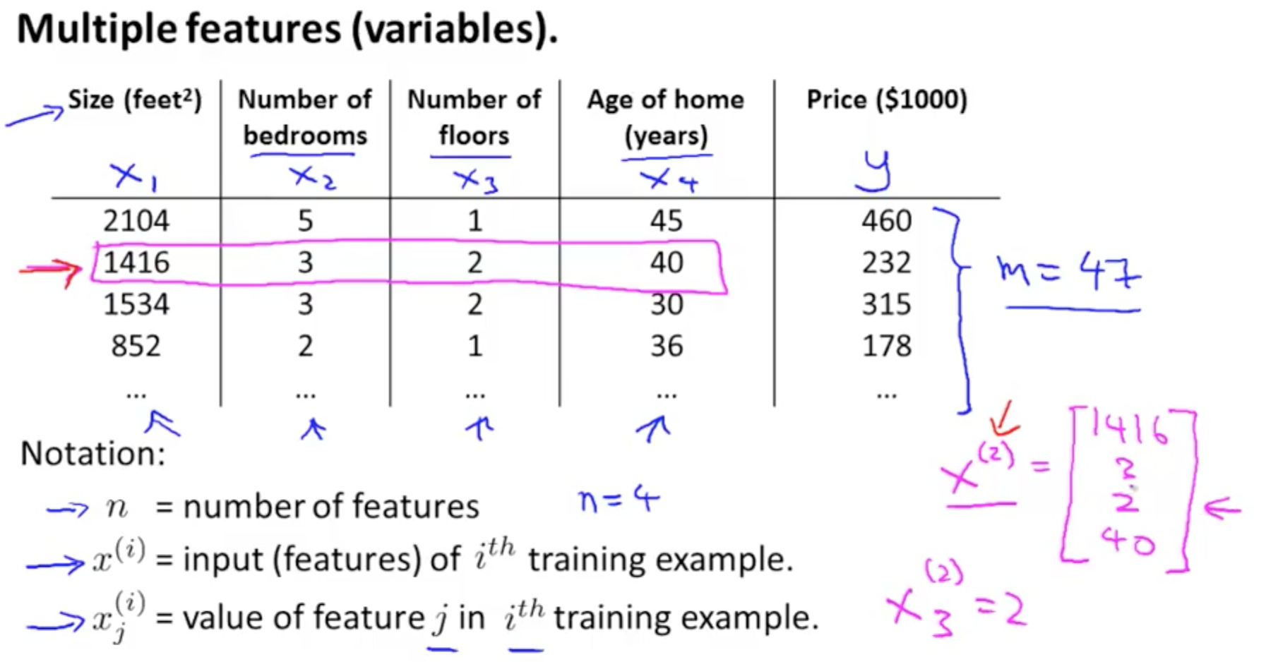
Note that m = number of training examples. If we have data of 1000 different houses, m=1000. In the picture above, there are 4 features so n=4. To speed up training, we store our dependent features in the form of a matrix X. 

X is a matrix with each row being one training example. Each column represents one feature.

We store our labels as a y vector of dimension m x 1. 

Hypothesis:

Our regression line consists of infinite points that try to best model the given data. For a given training example we make a prediction called a hypothesis, denoted by h(x) or ŷ, where: 

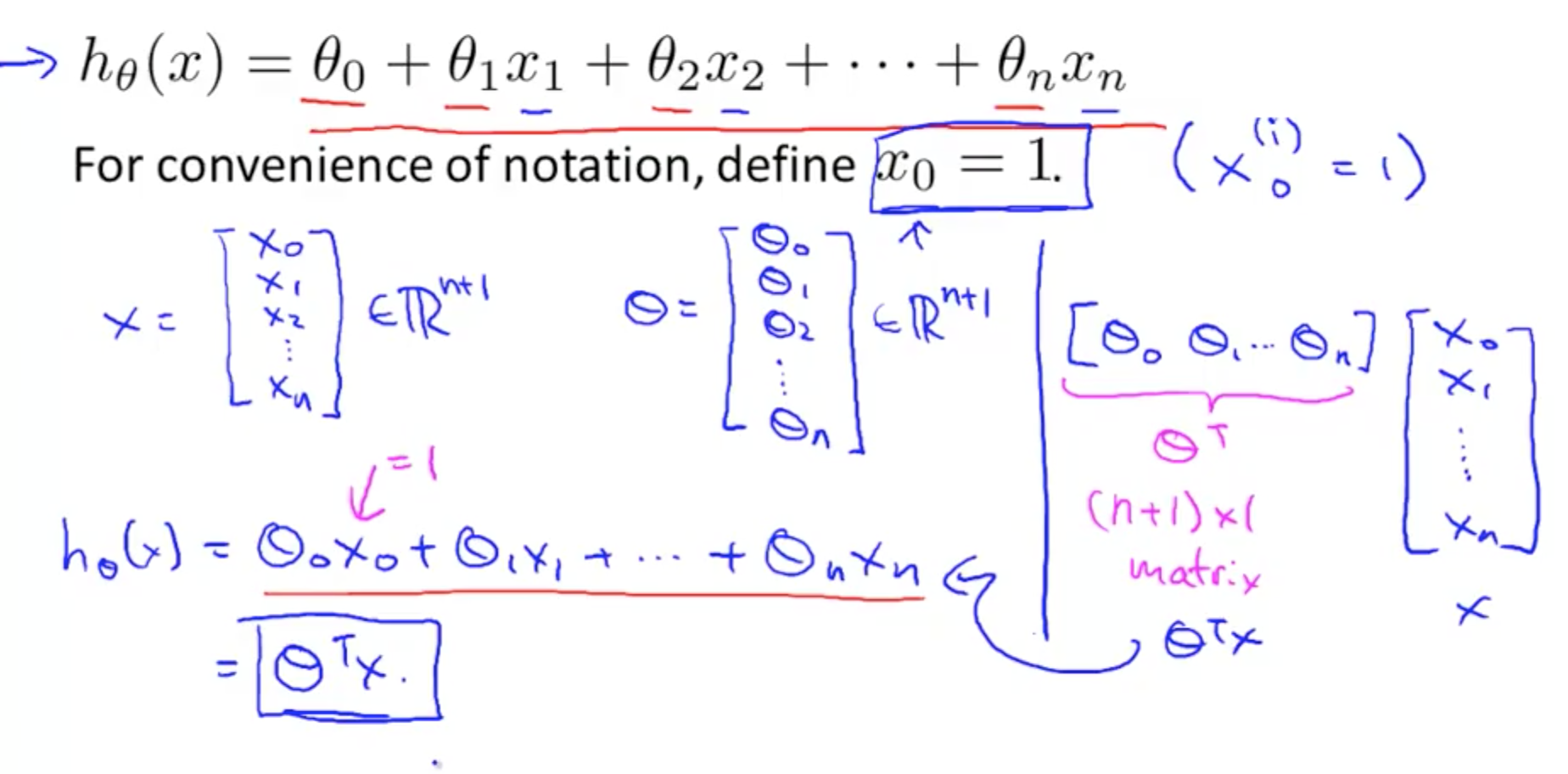
So, 

1. X is a matrix of size m x (n+1) 
2. θ is a vector of  (n+1)   x   1 

Vectorization:

The use of for loops while writing machine learning algorithms should be avoided as much as possible. To avoid this, we store data in the form of vectors or matrices and perform mathematical operations on them. This approach is much faster than the use of explicit for loop, almost more than 100 times! 

Here, to get all our predictions at once, we do the matrix multiplication Xθ, which returns all the hypotheses for all the training examples in the form of a vector of size m x 1.

Loss Function:

Now, a question...how do we decide our line of best fit? We must have an error metric to measure how well our model fits our data. The error metric is called our loss function, denoted by the letter J. Some common 

loss functions are:

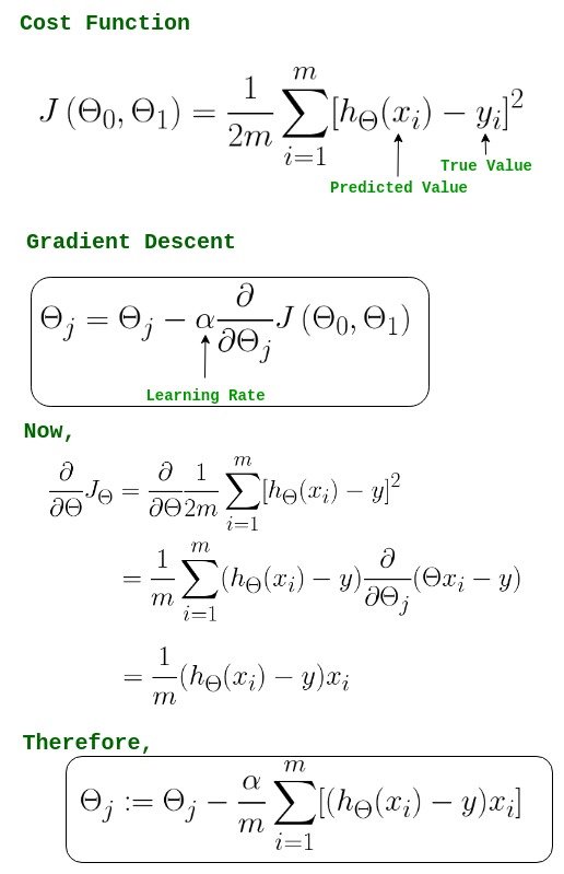
We will use one half the mean squared error as our error metric.

Gradient Descent:

And now comes the most important question...how do we obtain our parameters, that is, the theta vector? We use an optimization algorithm called gradient descent.

PLEASE NOTE THAT GRADIENT DESCENT IS A VERY IMPORTANT TOPIC IN MACHINE LEARNING AND DEEP LEARNING. HENCE WE ADVISE YOU TO GO THROUGH THE 4 VIDEOS GIVEN BELOW AND HAVE A THOROUGH UNDERSTANDING. FURTHER TOPICS WILL BE DIFFICULT TO UNDERSTAND IF THIS IS NOT UNDERSTOOD PROPERLY.

1) https://www.youtube.com/watch?v=F6GSRDoB-Cg&list=PLLssT5z_DsK-h9vYZkQkYNWcItqhlRJLN&index=8

2) https://www.youtube.com/watch?v=YovTqTY-PYY&list=PLLssT5z_DsK-h9vYZkQkYNWcItqhlRJLN&index=9

3) https://www.youtube.com/watch?v=GtSf2T6Co80&list=PLLssT5z_DsK-h9vYZkQkYNWcItqhlRJLN&index=10

4) https://www.youtube.com/watch?v=pkJjoro-b5c&list=PLLssT5z_DsK-h9vYZkQkYNWcItqhlRJLN&index=19

To summarize gradient descent, we repeat the following steps until we reach reasonably close to the minima:

Note that 𝛂 and the number of times we perform gradient descent are hyperparameters to be set by the user. To learn more about how to set these feel free to PM me or the others.